Analysis, Visualization and Mapping in R
Exercise 1: Produce a quick ready-to-share analysis using cepespata
Create a project in Rstudio.
Download a CSV from cepesp.io to your project folder. Use the ‘Eleicoes por Cargo’ tab with the default options. The file should include the results of the 2014 Presidential election aggregated for the whole of Brazil.
Create a new Rmarkdown document file.
Install and load the ‘tidyverse’ and ‘knitr’ packages
install.packages(c("tidyverse","knitr"))
library(tidyverse)
library(knitr)library(tidyverse)
library(knitr)- Import the CSV to Rstudio.
pres_2014_elec_results <- read_csv("TSE_PRESIDENTE_BR_CANDIDATO_2014.csv")- How many rows are there in the dataset?
pres_2014_elec_results %>% count()## # A tibble: 1 x 1
## n
## <int>
## 1 13- Note your dataset contains both the first and second rounds. How many candidates competed in the first round?
pres_2014_elec_results %>% filter(NUM_TURNO==1) %>%
count()## # A tibble: 1 x 1
## n
## <int>
## 1 11- How many people voted in the first round of the election?
voters_first <- pres_2014_elec_results %>%
  filter(NUM_TURNO==1) %>%
  summarize(Total_Votes=sum(QTDE_VOTOS)) %>%
pull(Total_Votes)## [1] 104023802- What was the percentage increase in the total number of people who voted between the first and second round? Use an in-line code expression.
voters_second <- pres_2014_elec_results %>%
  filter(NUM_TURNO==2) %>%
  summarize(Total_Votes=sum(QTDE_VOTOS)) %>%
  pull(Total_Votes)

pct_change <- 100*(voters_second - voters_first)/voters_firstThe percentage increase in the total number of people who voted between the first and second round was 1.5%.
- The data contains only the number of votes. Calculate the vote share of each candidate for each round as a new column in your data frame. (Remember to assign the result as an object we can use for the rest of the exercise).
pres_2014_elec_results <- pres_2014_elec_results %>%
  group_by(NUM_TURNO) %>%
mutate(Vote_Share=100*(QTDE_VOTOS/sum(QTDE_VOTOS)))## # A tibble: 13 x 3
## # Groups: NUM_TURNO [2]
## NUM_TURNO NOME_CANDIDATO Vote_Share
## <int> <chr> <dbl>
## 1 1 MAURO LUÍS IASI 0.0460
## 2 1 RUI COSTA PIMENTA 0.0118
## 3 1 JOSÉ LEVY FIDELIX DA CRUZ 0.430
## 4 1 MARIA OSMARINA MARINA DA SILVA VAZ DE LIMA 21.3
## 5 1 EVERALDO DIAS PEREIRA 0.750
## 6 1 AÉCIO NEVES DA CUNHA 33.5
## 7 2 AÉCIO NEVES DA CUNHA 48.4
## 8 1 JOSE MARIA EYMAEL 0.0589
## 9 1 LUCIANA KREBS GENRO 1.55
## 10 1 JOSÉ MARIA DE ALMEIDA 0.0877
## 11 1 DILMA VANA ROUSSEFF 41.6
## 12 2 DILMA VANA ROUSSEFF 51.6
## 13 1 EDUARDO JORGE MARTINS ALVES SOBRINHO 0.606- Insert an ‘in-line’ sentence that explains which candidate won the election and what percentage of the vote they received.
winner <- pres_2014_elec_results %>%
  filter(NUM_TURNO==2) %>%
  arrange(-Vote_Share) %>%
  slice(1) %>%
  select(SIGLA_PARTIDO, NOME_CANDIDATO, Vote_Share)

winner_name <- winner %>% pull(NOME_CANDIDATO)
winner_Votes <- winner %>% pull(Vote_Share)The winner was DILMA VANA ROUSSEFF with 51.6% of the vote.
- Produce a table which shows the results of the first round of the election, including vote share, but excluding boring columns like the year, candidate number etc.
pres_2014_elec_results %>%
  filter(NUM_TURNO==1) %>%
  select(NOME_CANDIDATO, SIGLA_PARTIDO, Vote_Share) %>%
kable()NUM_TURNO NOME_CANDIDATO SIGLA_PARTIDO Vote_Share ———- ——————————————- ————– ———– 1 MAURO LUÍS IASI PCB 0.0459943 1 RUI COSTA PIMENTA PCO 0.0118473 1 JOSÉ LEVY FIDELIX DA CRUZ PRTB 0.4295921 1 MARIA OSMARINA MARINA DA SILVA VAZ DE LIMA PSB 21.3187930 1 EVERALDO DIAS PEREIRA PSC 0.7503215 1 AÉCIO NEVES DA CUNHA PSDB 33.5473328 1 JOSE MARIA EYMAEL PSDC 0.0588808 1 LUCIANA KREBS GENRO PSOL 1.5498241 1 JOSÉ MARIA DE ALMEIDA PSTU 0.0876809 1 DILMA VANA ROUSSEFF PT 41.5940075 1 EDUARDO JORGE MARTINS ALVES SOBRINHO PV 0.6057258
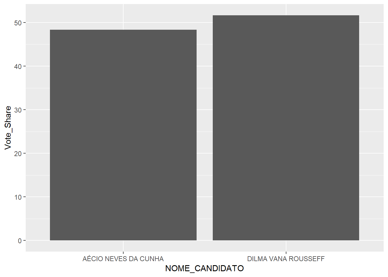
- Produce a bar chart which shows the results of the second round of the election by vote share.
pres_2014_elec_results %>%
  filter(NUM_TURNO==2) %>%
  ggplot() +
  geom_col(aes(x=NOME_CANDIDATO,y=Vote_Share))
- Specify whether you want the processing code to show up in your final document.
#Place this line in a chunk at the start of your code to make sure only the outputs appear
opts_chunk$set(echo=FALSE, warning=FALSE, message=FALSE)
Produce a PDF which combines all your outputs (text, table, chart).
Produce a web page which combines all your outputs (text, table, chart).
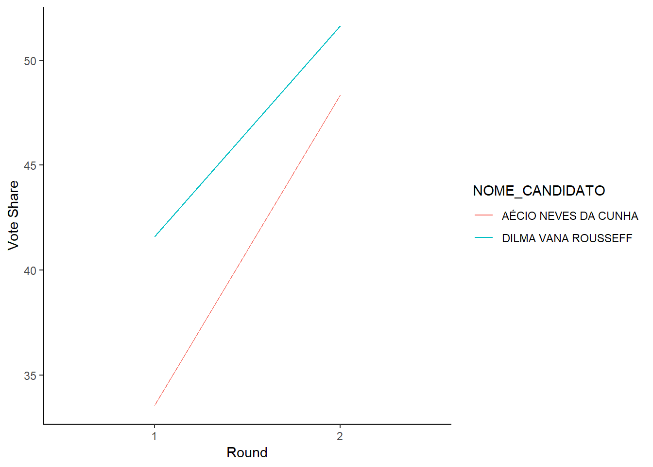
(If you have time…) Include a line chart which shows how the vote share of the two candidates that made the second round changed from the first to the second round.
runoff_cands <- pres_2014_elec_results %>%
  filter(NUM_TURNO==2) %>%
  pull(NUMERO_CANDIDATO)

pres_2014_elec_results %>% filter(NUMERO_CANDIDATO %in% runoff_cands) %>%
  ggplot() + geom_line(aes(x=as.factor(NUM_TURNO),y=Vote_Share,group=NOME_CANDIDATO,color=NOME_CANDIDATO)) +
  theme_classic() +
  xlab("Round") +
  ylab("Vote Share")